Principal Directions
This tutorial probes the tensor state (e.g., stress, strain) of a model at a site and plots the
principal directions on a stereonet. The principal_directions job:
Extracts a spherical site from the model.
Averages the tensors of the cells inside.
Computes the principal directions of the averaged tensor.
Transforms them to trend and plunge.
Plots them as \(\sigma_1 \leq \sigma_2 \leq \sigma_3\), with \(\sigma_1\) the most compressive.
The principal_directions job helps identify the tensor orientation at a site and the scatter
of the cells located in the extracted sphere.
The model
The input model is a finite element external simulation of a reverse fault with an elasto-plastic rheology, loaded in compression. The fault accommodates slip as a weak interface inside the medium. The figure below shows the geometry and boundary conditions.

Right: Geometry and boundary conditions of the model. Left: Displacement field and the spherical site.
Basic
A minimal configuration only needs the job name, a schema, a model file, and a site:
job: principal_directions
schema: adeli3
model: ../data/reverse_fault.vtu
site: {center: [10000, 5000, -2500], radius: 200}
output:
  dir: ./
Run it with:
$ fem2geo a_basic.yaml
The result is a stereonet with the three average principal directions of the sphere.
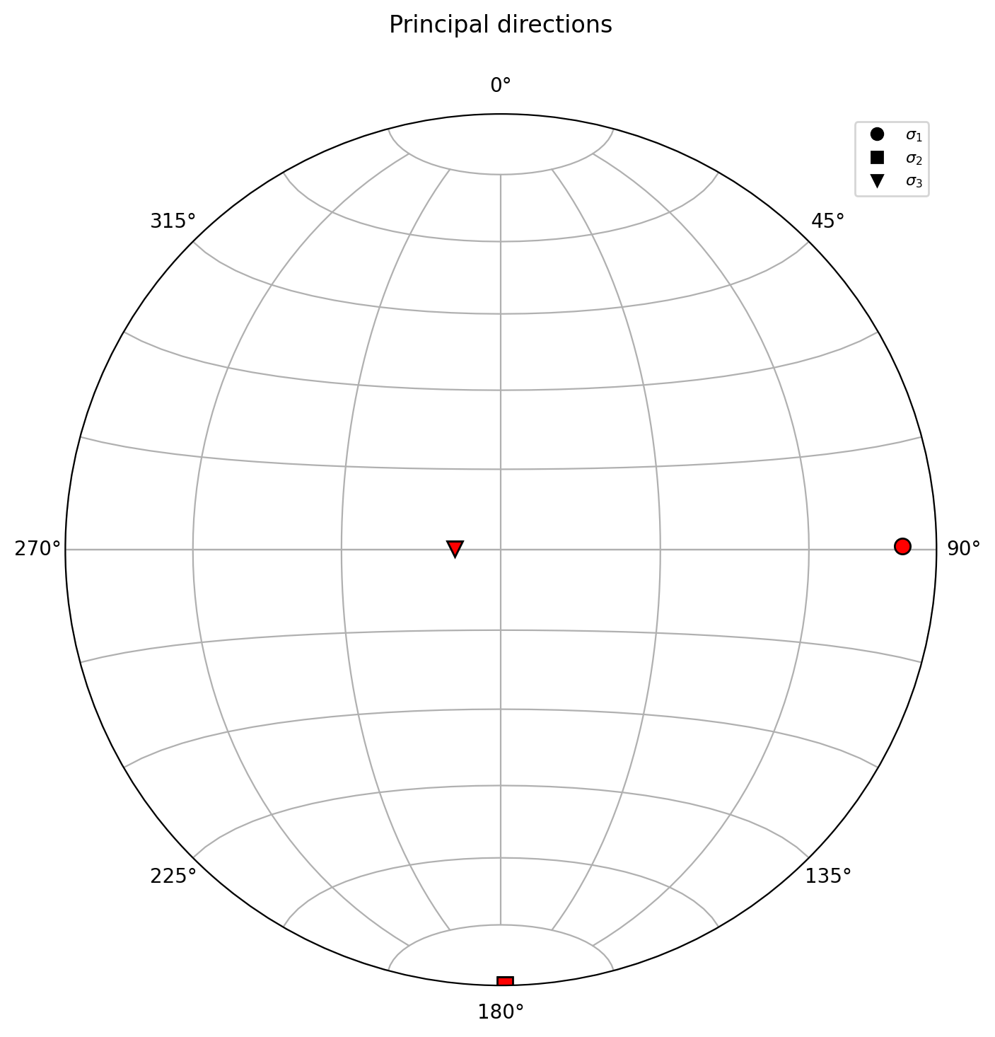
Average principal directions at the selected site.
Styled
The styled configuration analyzes de strain tensor, adds a title, figure size, and displays the per-cell directions as a scatter cloud around the average:
job: principal_directions
schema: adeli3
model: ../data/reverse_fault.vtu
tensor: strain
site: {center: [10000, 5000, -2500], radius: 200}
plot:
  title: "Principal strain directions"
  figsize: [8, 8]
  dpi: 300
  principals:
    color: "red"
    markersize: 10
  cell_principals:
    show: true
    style: scatter
    markersize: 2
    alpha: 0.2
output:
  dir: scatter/
  figure: principal_scatter.png
  vtu: sphere.vtu
Run it with:
$ fem2geo b_styled.yaml
The scatter cloud gives an idea of how coherent the stress field is inside the sphere. A tight cluster around the average means the principal directions are consistent across cells; a wide spread suggests the site is located in a transition.
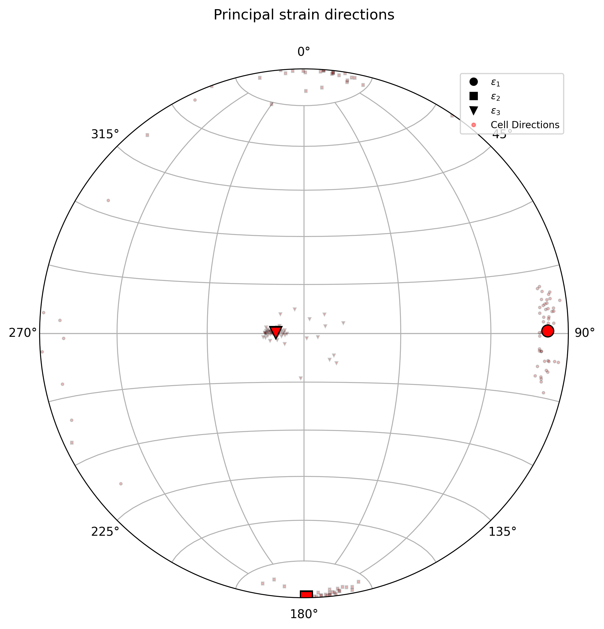
Average directions with cell-wise scatter.
Contours instead of scatter
When the site has many cells, scatter points pile up and become hard to read.
Switching to contour style draws density contours instead:
cell_principals:
  show: true
  style: contour
  levels: 4
  sigma: 2
  linewidth: 1.5
levels controls how many contour lines are drawn; sigma controls the
kernel bandwidth of the density estimate.
Multiple sites
To probe several sites at once — for example along a borehole — use the
sites dispatcher. See Multiple Sites for details.
Understanding the configuration
Job and schema
job: principal_directions
schema: adeli
job picks the workflow. schema maps solver-specific field names.
Note
The schema tells fem2geo how to find stress, strain, and other
fields in your model file, since different solvers store them under
different names. Built-in schemas are included in fem2geo to cover the
common cases. See User Guide for the full list and how to
write your own.
Tensor
By default the job analyses the stress tensor. To analyse a different tensor
(strain, strain rate, etc.), set tensor at the top level:
tensor: strain
Model input
model: ../data/reverse_fault.vtk
Path is relative to the config file.
Site
site: {center: [10000, 5000, -2500], radius: 200}
The site is a sphere. center places it in model coordinates; radius
controls how many cells are averaged. Smaller radii give a more local
measurement, larger radii average over a wider region.
Plot options
The plot block groups everything that affects the figure:
plot:
  title: "Principal stress directions"
  figsize: [9, 9]
  dpi: 300
  legend_size: 8
  legend_loc: "best"
  principals:
    color: "red"
    markersize: 10
  cell_principals:
    show: true
    style: scatter
    markersize: 3
    alpha: 0.3
title,figsize,dpi— figure-level.legend_sizeandlegend_loc— legend scaling and position.locaccepts"best",1,2,3,4.principals— style for the three average axes. Always drawn.cell_principals— per-cell scatter or density contours. Off by default.
Two cell styles are available:
scatter— one marker per cell.contour— kernel density contours. Extra keyslevels,sigma,linewidth.
Output
output:
  dir: scatter/
  figure: principal_directions.png
  vtu: extract.vtu
dir is the output folder (created if missing). figure is the figure
filename. vtu is optional; when present, the extracted sphere is saved
as a VTU file for inspection in Paraview.