User Guide
Overview
fem2geo is a tool for structural geology analyses on the output of FEM
and BEM models. The workflow has the same shape for most analyses:
Load a model from a solver output file (usually a
.vtu).Extract a region of the model — a sphere around a point of interest.
Compute a geomechanical quantity from the tensors inside that region: principal directions, slip or dilation tendency, resolved shear, etc.
Load data from a table, rasters, shapefiles or an additional
.vtu.Plot the result, usually on a stereonet, and optionally save the extracted region as a
.vtufile for inspection in Paraview.
There are two ways to drive this workflow. The main way is a YAML config file run from the command line, which is what the tutorials cover. The other is Python scripting, which is useful for advanced exploration and custom analyses (See Jupyter notebooks)
Model Data
A model is a mesh of cells, each carrying the physical quantities produced by the solver: stress and strain tensors, displacement, velocity, plastic strain, tensor invariants, etc.
Different solvers use different array names. A stress tensor could be stored as six separate
scalars (Stress_xx, Stress_yy, …), or packed as a single Voigt array (stresses_(Pa)),
or already decomposed into principal values and directions. The schema maps these
solver-specific names to a single set of canonical names that fem2geo uses everywhere.
Once a model is loaded with the right schema, fem2geo can work with the model.
fem2geo ships built-in schemas. For other solvers, writing a YAML file is required, which
can be easily derived from existing schemas.
Stereonets
Most fem2geo plots are stereonets. A stereonet is a flat disc that shows the lower half of a
sphere, seen from above.

A line through the centre of the sphere hits the bowl at one point. Projecting that point in the horizontal, gives a line in the stereonet (right). A line is defined by a trend (\(\alpha\)) and plunge (\(\beta\)).
fem2geo uses the lower-hemisphere equal-area (Schmidt)
projection. North is at the top, azimuth goes clockwise, the edge of
the disc is horizontal, and the centre is straight down. Three kinds of things show up on a
stereonet.
Points are lines. A principal stress direction, the pole of a plane, a slip vector — each is one point.
Great circles are planes. A fault or a fracture plane is drawn as a curve running from edge to edge. The pole of the plane is the point 90° away from the curve.

A plane in 3D is one curve on the disc. A plane is defined by a strike (\(\rho\)) and dip (\(\delta\)).
Stereo-contours are scalar fields that depend on orientation.
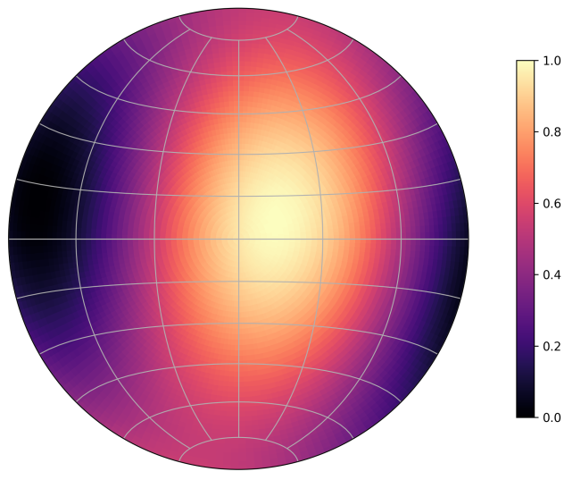
For every possible line orientation in the stereoplot, a colour shows the value of the scalar field.
Conventions
Model frame
Models usually live in a right-handed Cartesian frame. These can be:
A frame with X = East, Y = North, Z = Up and arbitrary origin.
A rotated local frame for convenience, with X and Y in the horizontal
An specific projected Coordinate Reference Systems (CRS), such as UTM19S, etc.
Units are whatever the solver used. fem2geo does not rescale. When extracting a sub-region from a model
site centres and radii must be in the same units as the model.
If the model or data is georeferenced (data in lon/lat, a model in projected CRS, a DEM), the model
is in a local and/or rotated frame, the project job can reproject real data onto the model
frame first.
Stress and strain
In most models, stresses and strains follow the continuum mechanics sign convention, with tension and extension taken as positive. This is in contrast to a geomechanical convention, where compression/contraction have negative sign.
Internally, fem2geo assumes:
Compression is negative. A uniaxial compression along X gives a negative
stress[0, 0]. Similarly, shortening is negative in strain.
The continuum mechanics convention (in contrast to geology or geotechnical) makes tension positive and compression negative. A normal stress is positive when it acts in the positive coordinate direction on a positive face (outward normal along +axis).
Principal values and directions are sorted in ascending order. Index 0 is the most compressive (stress) or most shortening (strain), index 2 is the least.

The stress tensor \(\boldsymbol{\sigma}\) has three orthogonal eigenvectors: \(\boldsymbol{\sigma}_1\), \(\boldsymbol{\sigma}_3\), \(\boldsymbol{\sigma}_3\). along which the stress is purely compressive or tensile (with no shear). In continuum mechanics the ordering is according to the associated eigenvalues, with \(\sigma_1 \geq \sigma_2 \geq \sigma_3\), so \(\sigma_3\) is the most compressive and \(\sigma_1\) the least.
However, fem2geo resulting stereoplots are always in geology convention:
Warning
Compression is positive in fem2geo stereoplots
This meant to be consistent with the geological literature. For instance \(\sigma_1\) is the most compressive stress and \(\varepsilon_1\) is the most contractional strain.
Planes and lines
Strike (\(\rho\)) is measured clockwise from North, in degrees.
Dip (\(\delta\)) is the steepest angle of the plane, 0 (horizontal) to 90 (vertical). Dip falls to the right of the strike direction (right-hand rule).
Trend (\(\alpha\)) and plunge (\(\beta\)) describe lines. Trend is the azimuth from North, plunge is the downward angle from horizontal.
Note
See Stereonets for a visual guide of the plane and lines convention.
Rake (\(\lambda\)) is the angle of the slip vector measured along the fault plane, starting from the strike direction, in Aki & Richards convention.
The Aki & Richards (1980) convention
Rake is measured along the fault plane from the strike counter-clockwise, taking values between -180 and 180. Positive rake means the hanging wall moved up along the slip direction (reverse/thrust component). Negative rake means a normal faulting component. A rake of 0° is pure left-lateral strike slip, 90° is pure reverse, 180° (or −180°) is pure right-lateral, and −90° is pure normal.

Schematic of the Aki & Richards rake convention.
CSV data
Structural CSVs have named columns:
Fractures need
strikeanddip.Faults need
strike,dip, andrake.Catalogs need
longitude,latitude, anddepthby default; the column names are configurable.
Configuration files
The core usage of fem2geo is through configuration files. These define the standardized
functionality of the package, which allows reproducibility of the analyses.
A config file looks like this:
job: principal_directions
schema: adeli3
model: ../data/reverse_fault.vtu
site:
   center: [10000, 5000, -2500]
   radius: 200
output:
  dir: ./
Run it from the command line:
$ fem2geo basic.yaml
Paths inside the config are relative to the config file, so you can move a config and its data around together without breaking anything. Every config has the same top-level keys. Most are shared across jobs.
job
The analysis to run. One of:
principal_directions— principal stress or strain directions at a site. See Principal Directions.fracture— compare fracture measurements against model principal directions. See Fracture Analysis.resolved_shear— compare observed fault slip against model-predicted slip. See Resolved-Shear Analysis.kostrov— compare a Kostrov moment tensor from faults against the model tensor. See Kostrov-Tensor Analysis.tendency— slip, dilation, or summarized tendency fields. See Tendency Plots.sites.<inner>— run any of the above over several sites at once on one figure, e.g.sites.tendency,sites.fracture. See Multiple Sites.project— reproject georeferenced data into the model’s local frame. See Projecting onto a Model Frame.
schema
Maps solver-specific array names to canonical names. Pick a built-in:
# TODO: well-define latest adeli schema.
model
Path to the solver output file, usually a .vtu. Relative to the
config.
tensor
Which tensor the analysis should use. Jobs that work on tensor data accept:
stress— total Cauchy stress.stress_dev— deviatoric stress.strain— total strain.strain_rate— strain rate.strain_plastic— plastic strain.strain_elastic— elastic strain.
site (or sites)
Where on the model the analysis happens. A site is a sphere, with a centre and a radius:
site:
  center: [10000, 5000, -2500]
  radius: 200
The radius controls how many cells the tensor is averaged over. Smaller
radius, more local. Larger radius, smoother average. Jobs that compare
against structural data also carry a data key with a CSV path:
site:
  center: [10000, 5000, -2500]
  radius: 500
  data: ../data/fractures.csv
For multi-site runs, use sites and list them by name:
sites:
  north:
    center: [10000, 8000, -2500]
    radius: 500
  south:
    center: [10000, 2000, -2500]
    radius: 500
    title: "Southern block"
plot
Everything that controls how the figure looks: title, figure size, DPI, legend size and location, colors and marker sizes for each element. The exact keys depend on the job — every job documentation page lists its own plot block in full.
output
Where to save results.
output:
  dir: results/
  figure: my_plot.png
  vtu: extract.vtu
The folder is created if it does not exist. The figure key is
optional; each job has a default filename. The vtu key is optional
too; when present, the extracted sphere is saved so it can be opened in
Paraview.
Schemas
A schema tells fem2geo where to find things inside a solver output
file. Different solvers use different names for the same quantities:
one could call the stress tensor stress, and other stresses. Another solver could split
it into six values stress_xx, stress_yy, etc. The
schema maps these names to the standard names that fem2geo uses
everywhere.
Built-in schemas
fem2geo ships with schemas for the Adeli solver:
schema: adeli
Writing your own
A schema has two parts:
tensors— the stress, strain, or other 3×3 tensors.fields— everything else (scalars and vectors).
Most jobs need at least one tensor, usually stress. The exception is
project, which does not touch tensor data.
There are two ways to give fem2geo a schema.
Write it in a separate file and point the config at it:
schema: ./my_solver.yaml
The file looks like this:
solver: my_solver

tensors:
  stress:
    voigt6: "stresses_(Pa)"

fields:
  u: { field: "displacement" }
Or write it directly in the config for a one-off run:
job: principal_directions
schema:
  solver: my_solver
  tensors:
    stress:
      voigt6: "stresses_(Pa)"
  fields:
    u: { field: "displacement" }

model: ../data/run.vtu
site: {center: [0, 0, -1000], radius: 200}
Use a separate file when you run many configs against the same solver. Use the inline form for quick tests.
Writing a tensor
A tensor entry has one of two shapes.
If the solver packs all six components into one array:
stress:
  voigt6: "stresses_(Pa)"
voigt6 is the name of the array in the solver file. The six values
must be in the order xx, yy, zz, xy, yz, zx.
If the solver stores one array per component:
stress:
  components:
    xx: "Stress_xx(MPa)"
    yy: "Stress_yy(MPa)"
    zz: "Stress_zz(MPa)"
    xy: "Stress_xy(MPa)"
    yz: "Stress_yz(MPa)"
    zx: "Stress_zx(MPa)"
The names fem2geo recognises for tensors are: stress,
stress_dev, strain, strain_rate, strain_plastic,
strain_elastic. Only list the ones your solver saves.
Writing a scalar/vector field
Fields are scalars or vectors. Each entry maps a standard name to the solver’s array name:
fields:
  u:      { field: "displacement" }
  plastic_eff:      { field: "effective_plastic_strain" }
  plastic_vol:      { field: "plastic_dilation" }
The standard names fem2geo knows about include:
u,v— displacement and velocity.plastic_eff,plastic_vol— plastic strain scalars.
Arrays in the solver output that the schema does not list are ignored. You only have to map the ones your analysis will use.
Python API
Everything above can be done directly from Python, without a config file. This is the path for exploration, custom plots, and analyses that do not fit any of the built-in jobs.
The Python API is covered in the notebook tutorials (coming soon). They
walk through loading a model, extracting regions, calling the tensor
primitives directly, and embedding fem2geo stereonets inside custom
matplotlib figures.
See also
Theory — mechanical and structural geology background.
API Documentation — full function reference.