Comparing Two Models

Load two solver runs of the same region: a reverse-fault experiment and a normal-fault experiment. Plot their principal directions on one stereonet. Then overlay a fracture population and see which model is more consistent with the measurements.

Setup

import os

import matplotlib.pyplot as plt
import mplstereonet  # noqa: F401

from fem2geo import Model, dir_testdata
from fem2geo.internal.io import load_structural_csv
from fem2geo.plots import stereo_axes, stereo_pole

Loading two models

Both files live in the tutorials data directory. They use the same schema.

reverse = Model.from_file(
    os.path.join(dir_testdata, "reverse_fault.vtu"), schema="adeli3"
)
normal = Model.from_file(
    os.path.join(dir_testdata, "normal_fault.vtu"), schema="adeli3"
)

print("reverse:", reverse.n_cells, "cells")
print("normal: ", normal.n_cells, "cells")

reverse: 52388 cells
normal:  42106 cells

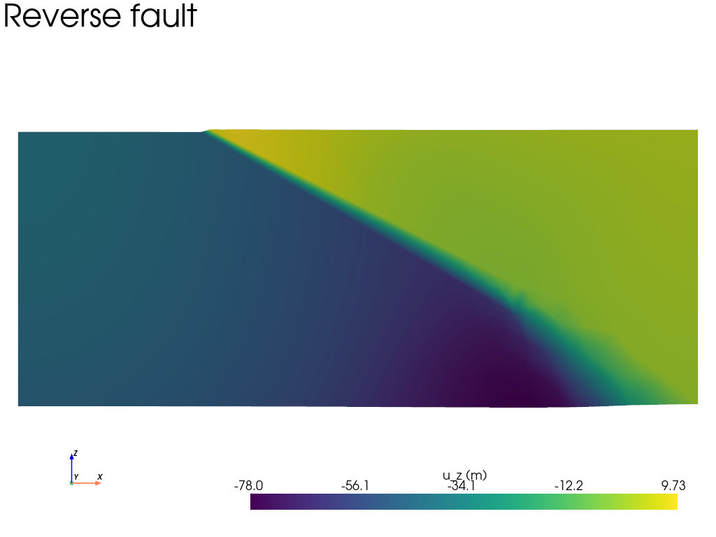
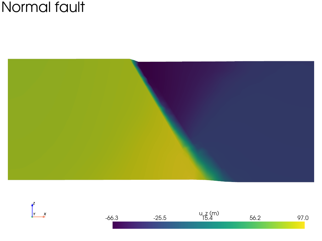
We plot a slice for each model at the same place.

sl = reverse.grid.slice(normal="y", origin=(0, 5000, 0))
sl.plot(
    scalars="u",
    component=2,
    cpos="xz",
    zoom=1.4,
    text="Reverse fault",
    scalar_bar_args={"title": "u_z (m)"},
)

sl = normal.grid.slice(normal="y", origin=(0, 5000, 0))
sl.plot(
    scalars="u",
    component=2,
    cpos="xz",
    zoom=1.4,
    text="Normal fault",
    scalar_bar_args={"title": "u_z (m)"},
)

• 
• 

Picking a common site

The two models share the same geometry, so the same center and radius work for both.

center = [8000, 6000, -1500]
radius = 300

site_rev = reverse.extract(center=center, radius=radius)
site_nor = normal.extract(center=center, radius=radius)

Principal stress in both models

One call per model gives the eigenvalues and eigenvectors of the averaged stress tensor at the site. Since the site is the same, any difference is purely due to the loading conditions of each experiment.

_, vec_rev = site_rev.avg_principals("stress")
_, vec_nor = site_nor.avg_principals("stress")

Both on one stereonet

Drop both sets of axes into the same stereonet with different colors.

fig = plt.figure(figsize=(7, 7))
ax = fig.add_subplot(111, projection="stereonet")
ax.grid(True)

stereo_axes(
    ax, vec_rev,
    style={"color": "red", "markersize": 12},
    labels=(r"$\sigma_1$ reverse", r"$\sigma_2$ reverse", r"$\sigma_3$ reverse"),
)
stereo_axes(
    ax, vec_nor,
    style={"color": "blue", "markersize": 12},
    labels=(r"$\sigma_1$ normal", r"$\sigma_2$ normal", r"$\sigma_3$ normal"),
)
ax.legend()
ax.set_title("Principal stress: reverse vs normal", y=1.08)

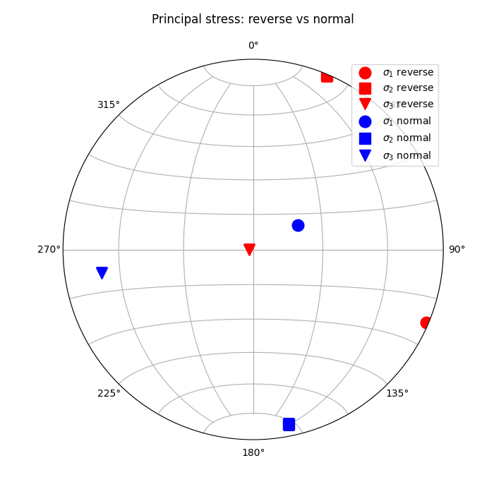
Text(0.5, 1.08, 'Principal stress: reverse vs normal')

Loading fracture measurements

A CSV with strike and dip columns becomes a FractureData object via load_structural_csv. The .planes attribute is a (N, 2) numpy array of [strike, dip].

fractures = load_structural_csv(
    os.path.join(dir_testdata, "fractures_c.csv")
)
print(fractures)
print("shape:", fractures.planes.shape)

FractureData(20 measurements)
shape: (20, 2)

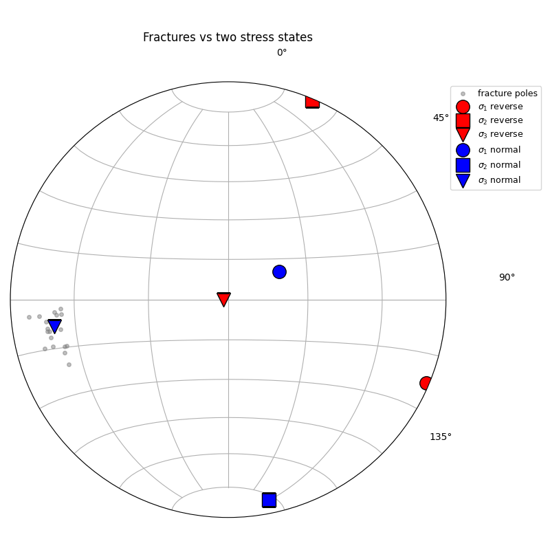
Fractures vs both models

Draw the fractures poles (one point per plane) and place the principal directions of each model on top. A fracture population that aligns with \(\sigma_3\) of a model is consistent with that stress state.

fig = plt.figure(figsize=(8, 8))
ax = fig.add_subplot(111, projection="stereonet")
ax.grid(True)

# fractures as poles
stereo_pole(
    ax, fractures.planes,
    marker="o", color="grey", markersize=4, alpha=0.5,
    label="fracture poles",
)

# reverse model principal directions
stereo_axes(
    ax, vec_rev,
    style={"color": "red", "markersize": 14, "markeredgecolor": "k"},
    labels=(r"$\sigma_1$ reverse", r"$\sigma_2$ reverse", r"$\sigma_3$ reverse"),
)

# normal model principal directions
stereo_axes(
    ax, vec_nor,
    style={"color": "blue", "markersize": 14, "markeredgecolor": "k"},
    labels=(r"$\sigma_1$ normal", r"$\sigma_2$ normal", r"$\sigma_3$ normal"),
)

ax.set_title("Fractures vs two stress states", y=1.08)
ax.legend(loc="upper left", bbox_to_anchor=(1.0, 1.0), fontsize=9)
plt.tight_layout()

/home/docs/checkouts/readthedocs.org/user_builds/fem2geo/checkouts/latest/tutorials/examples/02_comparing_models.py:162: UserWarning: This figure includes Axes that are not compatible with tight_layout, so results might be incorrect.
  plt.tight_layout()

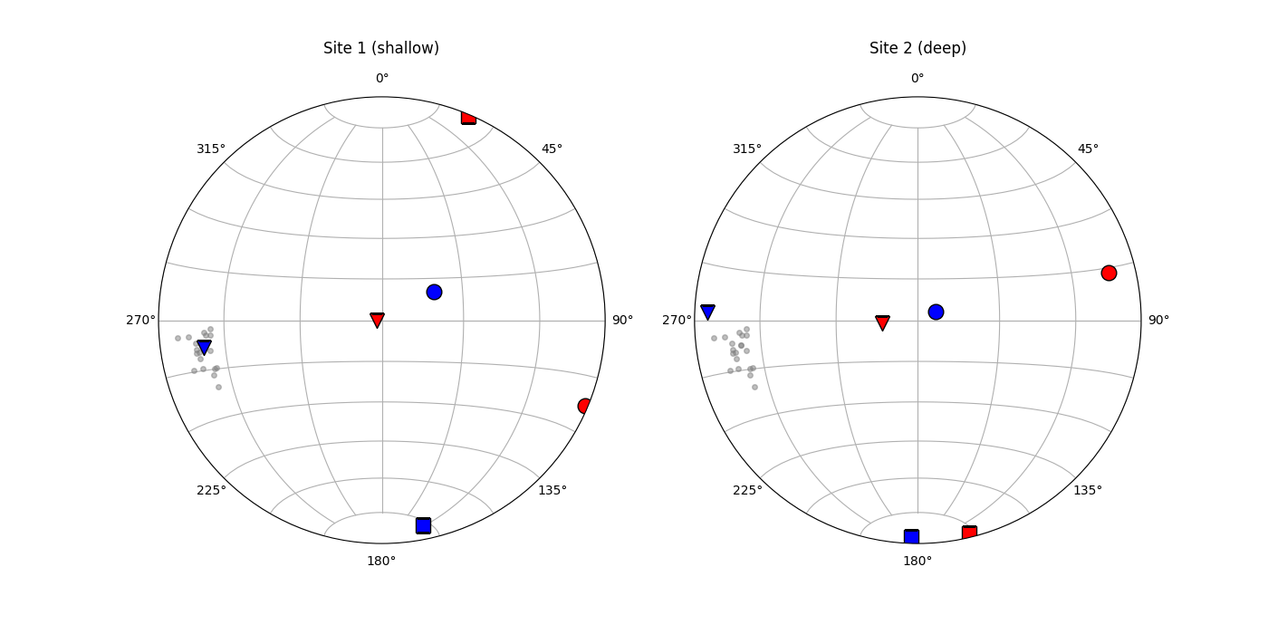
At multiple sites

Here are two sites side by side, each comparing the two models against the fractures.

sites_info = [
    ("Site 1 (shallow)", [8000, 6000, -1500]),
    ("Site 2 (deep)",    [8000, 6000, -2500]),
]

fig, axes = plt.subplots(
    1, 2, figsize=(14, 7),
    subplot_kw={"projection": "stereonet"},
)

for ax, (name, ctr) in zip(axes, sites_info):
    sub_r = reverse.extract(center=ctr, radius=radius)
    sub_n = normal.extract(center=ctr, radius=radius)
    _, vectors_r = sub_r.avg_principals("stress")
    _, vectors_n = sub_n.avg_principals("stress")

    ax.grid(True)
    stereo_pole(
        ax, fractures.planes,
        marker="o", color="grey", markersize=4, alpha=0.5,
    )
    stereo_axes(
        ax, vectors_r,
        style={"color": "red", "markersize": 12, "markeredgecolor": "k"},
        labels=(r"$\sigma_1$ rev", r"$\sigma_2$ rev", r"$\sigma_3$ rev"),
    )
    stereo_axes(
        ax, vectors_n,
        style={"color": "blue", "markersize": 12, "markeredgecolor": "k"},
        labels=(r"$\sigma_1$ nor", r"$\sigma_2$ nor", r"$\sigma_3$ nor"),
    )
    ax.set_title(name, y=1.08)

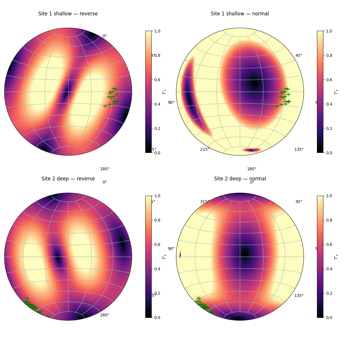
Slip tendency for two fault sets

Each model has its own stress state at each site. We plot the slip tendency field of that stress state as a stereonet contour, then overlay the observed fault poles on top.

from fem2geo.plots import stereo_field
from fem2geo.utils.tensor import slip_tendency
from fem2geo.utils.transform import grid_nodes, grid_centers

faults_a = load_structural_csv(os.path.join(dir_testdata, "faults.csv"))
faults_b = load_structural_csv(os.path.join(dir_testdata, "faults_b.csv"))

ms, md = grid_nodes(180, 45)
cs, cd = grid_centers(ms, md)

fig, axes = plt.subplots(
    2, 2, figsize=(12, 12),
    subplot_kw={"projection": "stereonet"},
)

cases = [
    ("Site 1 shallow", [8000, 6000, -1500], faults_a),
    ("Site 2 deep",    [8000, 6000, -2500], faults_b),
]

for row, (name, ctr, fd) in enumerate(cases):
    sub_r = reverse.extract(center=ctr, radius=radius)
    sub_n = normal.extract(center=ctr, radius=radius)
    T_r = sub_r.avg_tensor("stress")
    T_n = sub_n.avg_tensor("stress")

    ts_r = slip_tendency(T_r, cs.ravel(), cd.ravel()).reshape(cs.shape)
    ts_n = slip_tendency(T_n, cs.ravel(), cd.ravel()).reshape(cs.shape)

    for col, (vals, label) in enumerate([(ts_r, "reverse"), (ts_n, "normal")]):
        ax = axes[row, col]
        ax.grid(True)
        stereo_field(
            ax, ms, md, vals,
            cmap="magma", vmin=0.0, vmax=1.0,
            cbar=True, cbar_label=r"$T'_s$",
            cbar_kwargs={"shrink": 0.7},
        )
        stereo_pole(
            ax, fd.planes[:, 0], fd.planes[:, 1],
            marker="+", color="green", markersize=10,
        )
        ax.set_title(f"{name} — {label}", y=1.08)

plt.tight_layout()

/home/docs/checkouts/readthedocs.org/user_builds/fem2geo/checkouts/latest/tutorials/examples/02_comparing_models.py:256: UserWarning: This figure includes Axes that are not compatible with tight_layout, so results might be incorrect.
  plt.tight_layout()

---

GitHub | PyPI