Exploring a Model

Load a model, poke at what is inside, extract a region, and build a stereonet from scratch. No config files.

Setup

import os

import matplotlib.pyplot as plt
import mplstereonet  # noqa: F401

from fem2geo import Model, dir_testdata
from fem2geo.plots import stereo_axes

Loading a model

Model.from_file takes a path and a schema name. The schema says which solver format the file has

path = os.path.join(dir_testdata, "reverse_fault.vtu")
model = Model.from_file(path, schema="adeli3")

What is inside

print("cells:       ", model.n_cells)
print("points:      ", model.n_points)
print("u:           ", model.u.shape)
print("stress:      ", model.stress.shape)
print("j2_stress:   ", model.j2_stress.shape)

cells:        52388
points:       9783
u:            (9783, 3)
stress:       (52388, 3, 3)
j2_stress:    (52388,)

model.stress is a plain numpy array of shape (n_cells, 3, 3) Principal directions come as unit vectors. Displacement is a vector per cell. All the model attributes are regular arrays.

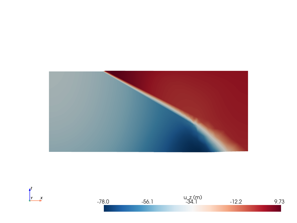
A horizontal slice of the whole model

model.grid is the underlying PyVista dataset. A horizontal slice at y=5000, colored by vertical displacement, shows where the fault zone is located.

sl = model.grid.slice(normal="y", origin=(0, 5000, 0))
sl.plot(
    scalars="u",
    component=2,
    cmap="RdBu_r",
    cpos="xz",
    scalar_bar_args={"title": "u_z (m)"},
)

Extracting a region

Analyses don’t use the whole model, but they are done on a site; e.g., a sphere around a point of interest. model.extract returns a new model restricted to the cells inside the sphere. It has the same interface as the original.

sub = model.extract(center=[8000, 5000, -2500], radius=300)
print(f"site: {sub.n_cells} cells out of {model.n_cells}")

site: 139 cells out of 52388

Average principal stress

avg_principals returns the eigenvalues and eigenvectors of the volume-weighted average tensor inside the site. Eigenvalues come sorted ascending, so index 0 is the most compressive.

values, vectors = sub.avg_principals("stress")
print("eigenvalues:", values)
print("eigenvectors (columns = sigma_1, sigma_2, sigma_3):")
print(vectors)

eigenvalues: [-132.90893237  -89.62799877  -56.67045117]
eigenvectors (columns = sigma_1, sigma_2, sigma_3):
[[-0.97426241 -0.01602738 -0.22484633]
 [-0.01724908  0.9998452   0.00347008]
 [ 0.22475591  0.00725916 -0.97438806]]

A stereonet

Plot functions in fem2geo.plots all take a matplotlib axes as the first argument and draw into it. You own the figure.

fig = plt.figure(figsize=(5, 5))
ax = fig.add_subplot(111, projection="stereonet")
ax.grid(True)

stereo_axes(
    ax, vectors,
    style={"color": "red", "markersize": 10},
    labels=(r"$\sigma_1$", r"$\sigma_2$", r"$\sigma_3$"),
)
ax.legend()
ax.set_title("Site 1 - principal stress", y=1.08)

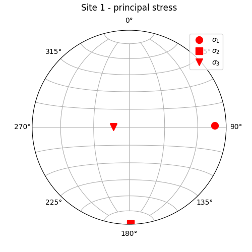
Text(0.5, 1.08, 'Site 1 - principal stress')

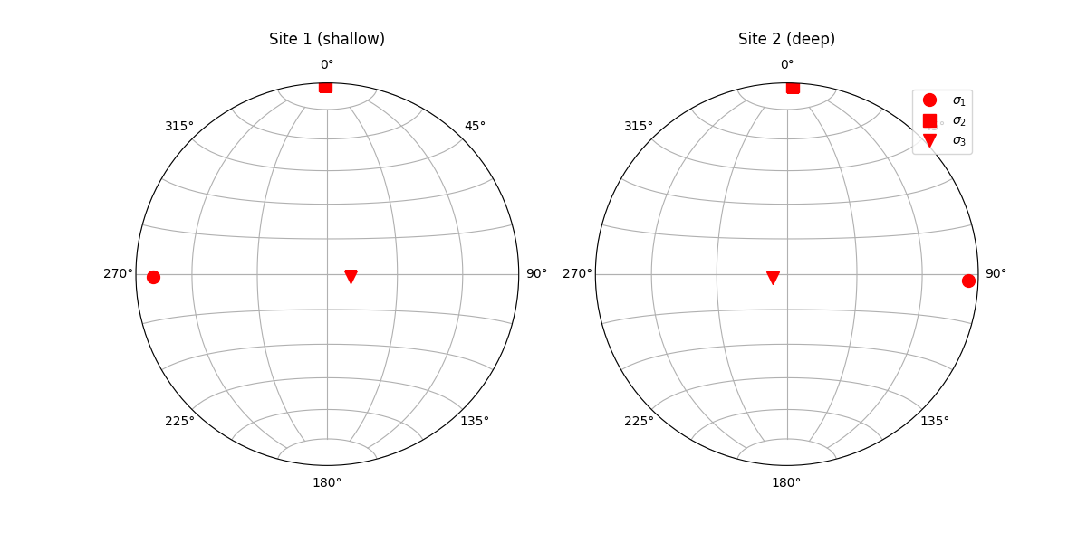
A second site, and a two-panel figure

Extracting more sites is just a loop. Placing them in a custom layout is just matplotlib.

sites = [
     model.extract(center=[8000, 5000, -2000], radius=300),
     model.extract(center=[8000, 5000, -4000], radius=300)]

site_names = ["Site 1 (shallow)", "Site 2 (deep)"]
fig, axes = plt.subplots(
    1, 2, figsize=(12, 6),
    subplot_kw={"projection": "stereonet"},
)

for ax, site, site_name in zip(axes, sites, site_names):
    _, vecs = site.avg_principals("stress")
    ax.grid(True)
    stereo_axes(
        ax, vecs,
        style={"color": "red", "markersize": 10},
        labels=(r"$\sigma_1$", r"$\sigma_2$", r"$\sigma_3$"),
    )
    ax.set_title(site_name, y=1.08)
ax.legend()

<matplotlib.legend.Legend object at 0x7bf67592ba50>

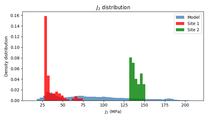
Other plots

Here are histograms of stress J2 in the model vs. the sites

j2_model = model.j2_stress
j2_site1 = sites[0].j2_stress
j2_site2 = sites[1].j2_stress

fig, ax = plt.subplots(figsize=(7, 4))
ax.hist(j2_model, bins="auto", color="steelblue", density=True, alpha=0.8,
        label="Model")
ax.hist(j2_site1, bins="auto", color="red", density=True, alpha=0.8, label="Site 1")
ax.hist(j2_site2, bins="auto", color="green",  density=True, alpha=0.8, label="Site 2")

ax.set_xlabel(r"$J_2$ (MPa)")
ax.set_ylabel("Density distribution")
ax.set_title(r"$J_2$ distribution")
ax.legend()
plt.tight_layout()

Saving the extracted site

The extracted subset is also a model. Save it to .vtu and open it in ParaView to see which cells were picked.

sites[0].save("site_1.vtu")

---

GitHub | PyPI